Global variables

Just the other day I was running a program in Simulink and I found a problem with global variables. The solution finally was really easy but I wanted to share it with you.

First of all, in order to initializate global variables, we can go to my previous post 'Clock Pulses Counter' where I explained how to do  it in detail.

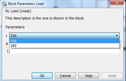
Back to the problem, I wanted to create an array of global variables in a Matlab function block. I realized that in order to do it, I just had to initializate the Data Store Memory into an array:

Array initialization Data Store Memory

Now, this global variable behaviours as an array.

Other thing I had to face was write and read a global variable out of a Matlab function block (in order to debug the code). Then I found some really interesting blocks: Data Store Read and Data Store Write, that allow us to read and write into the global variable.

Data Store Read

Data Store Write

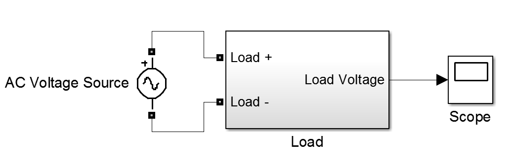
With that, I wanted to implement an example with both combinations: write and read global variables in a Matlab function block and write and read the same global variables with the Data Store Read and Data Store Write blocks.

The example I thought was to generate a 3-array and the values will be incremented by 1 or by 5 depending on the block reading and writing the global variables. The result was the following:

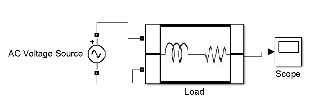
Example: General Block Diagram

Then, inside the 'Increment counter with Matlab function block' we can find the following blocks:

Matlab function block

By including the Trigger block or Enable block inside a subsystem we make the subsystem triggered or enabled by the outside. The code inside the block was:

function fcn

global counter_array;

global index;

if index < 3

    counter_array(index) = counter_array(index) + 5; %add 5 to the value 

    index = index +1;

else

    counter_array(index) = counter_array(index) + 5; %last index value

    index = 1;    

end

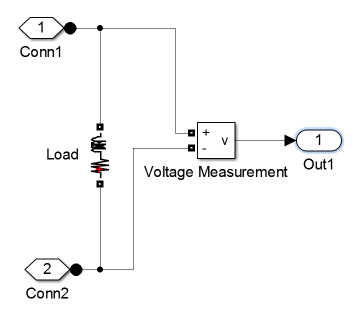
Inside the 'Increment counter reading and writing global variable' we can found the following blocks:

Increment counter reading and writing global variable block

Now, inside the 'Index < 3' block:

Index < 3 block

Here, depending on if the index is 1 or 2 we will develop different performances. 

In the case of Index ==1:

Enable Add1

The value inside array(1) will be increased by 1 and also the index:

Index++

In the case of index different from 1, we want to keep the array(1) and array(3) values, since we are changing index = 2, so the diagram block will be:

Enable Add~1

In the case of 'Enable Add 2' and 'Enable Add~2' is the same as the blocks before but changing array(1) to array(2). 

Nevertheless, in the case Index = 3, the block diagram will be the following:

Index = 3

And inside index = 1 block is just as simple as write a constant = 1 inside the Data Store Variable.

Index = 1

Finally, the theoretical result of that example should be:

Index = 1     Array[3] = [0,0,0]

Index = 2     Array[3] = [5,0,0]

Index = 3     Array[3] = [5,1,0]

Index = 1     Array[3] = [5,1,5]

Index = 2     Array[3] = [6,1,5]

Index = 3     Array[3] = [6,6,5]

Index = 1     Array[3] = [6,6,6]

Index = 2     Array[3] = [11,6,6]

Index = 3     Array[3] = [11,7,6]

...

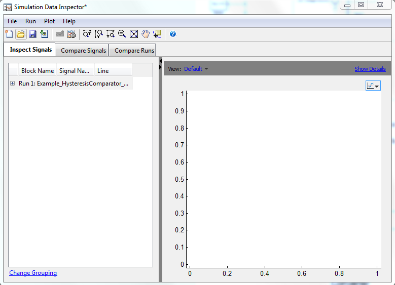
And the simulation we got was the following:

Example: Final Simulation

It can be seen that it is as expected.

Notice that is much more complicated read/write global variables with the 'Data Store Read' and 'Data Store Write' blocks than with the 'Matlab function' block. However, they are very useful in order to debug our code.

Hope this is useful and any comments with problems or recommendations are welcome!! See you soon!

Compare Simulink Data

This post is related with 'Export Simulink Data to Matlab' since it is another way to compare the simulink data. In the post 'Export Simulink Data to Matlab' we created variables in Matlab in order to process the data. In this post, I will explain how to easily compare some characteristics of variables in Simulink enviroment.

Let's took the same example as in 'Export Simulink Data to Matlab':

Export Simulink Data to Matlab Example

Now, we want to use the 'Test Points' to collect the data and the 'Signal Logging' to export that data. (This was explained in the 'Export Simulink data to Matlab' post.

Test Points and Signal Logging in signal wires.

Now, in order to initializate the Simulation Data Inspector, the button  must be clicked.

After running the simulation, the Simulation Data Inspector tab will appear:

Simulation Data Inspector tab

And after clicking 'Simulation Data Inspector' the following window will appear:

Simulation Data Inspector window

Here we can see the signals, look for a crossing points, and also compare signals with simulation with other parameters.

Example1: Let's exactly detect the crossing between the two signals we have.

In the Simulation Data Inspector, we can select the data cursor and detect the exact crossing of a run.

Croissing point 1

Crossing point 2

Example2: Let's compare the signal by changing a resistance value:

If we change R1 from 10kOhm to 20kOhm, the output signals will appear at the window:

Simulation Data Inspector - Inspect Signals

Here, we can select/deselect the signals in order to visually compare them.

Furthermore, at the compare Signals tab, we can select the signals we want to compare and the simulator will give us the difference and the tolerance between them.

Simulation Data Inspector - Compare Signals

Finally, we can select to compare runs at the Compare Runs tab and the simulator will plot the comparison between the same signals at the different runs.

Simulation Data Inspector - Compare Runs

We can use this tool to process some Simulink data in an easy way. If we want to perform more difficult functions to the data, I would export it to Matlab enviroment.

Hope this help and any comment will be welcome!

Mask a Subsystem

Once you have a subsystem created, there is the possibility of mask it.

Mask a subsystem could be useful in order to customized the block and make it more accessible to an external user.

Let's take a past example to modify it and demonstrate the mask application. First of all, we take the past post 'Create a Subsystem'. If we remeber this post, I created a simple subsystem of an LR Load.

Circuit inside subsystem

Load Subsystem

Now, let's mask the subsystem, customizing the previous image, and also adding some external parameters. The external parameters are useful to change the parameters on the circuit without getting inside it.

If we want to mask the subsystem, right-cliking the block, and selecting mask/create mask... or Ctrl + M when the block is selected. Then, the mask editor should open:

The mask editor allow us to change some of the subsytem options. For example, we can change the previous image of the subsystem in the first tab: Icon & Ports. Here, we can draw with Matlab plots, we can upload an image, etc.

In our case, let's take a simple image that represents our load:

RL Load

In order to upload to the subsystem, the image should be in a Matlab path or a known path. In our case, the image is inside the current directory.

Now, we program the command:

image (imread ('Load2','png'));

When we click apply, the changes can be seen:

Subsystem with image customized

Now, we are going to add some external parameters. Let's go to the Parameters pane:

Parameters tab

Button to add a parameter.


There are different kind of parameter types: edit, checkbox, popup, DataTypeStr, Minimum and Maximum. In this example we are going to use edit and popup.

In the case of the popup parameter, there is a list of options that we can choose. In the case of edit, any number could be added to the subsystem.

In our case, let's limit the L values options to 330H and 390H.

Notice that in 'Type-specific options' we have specified the options we want.

Now, after clicking apply, the subsystem would appear like the following:

Subsystem with mask

Now, in order to descend to the circuit, we have to click the arrow: 
When we normally click to the block, the window below will appear:

Subsystem window

Notice that the R parameter has to be entered, and we can choose L value between 330 and 390 H.

Subsystem window with popup

In order to make these parameters applicable in the circuit, we have to change the real values of R and L to our variables: 'L' and 'R':

Now, if an external user has to use the block, there is a mask to facilitate the options, like the different blocks in Simulink.

There is an initialization pane to initialize the mask block. Here we can add Matlab code that we like to run before the simulation starts.

Finally, lets add some information to the external users that can help them to understand our block. We can see a Documentation tab, where there are three sections: Mask type, Mask description, and Mask help.

Here, a explanation of the block must be added, in order to make it more understandable. The Mask type and Mask description will appear in the main window when we click the block. In we need more information, we could click the help button and the Mask help will appear:

Now, you can try with another type of parameters and options to make a more complicated subsystem. And comment the results here on the post! I will be glad to receive feedback and opinions!

Export Simulink Data to Matlab

In order to process the data on simulink models in Matlab enviroment, there is an easy way that convert Simulink signals into Matlab variables.

In order to explain it, let's take an example from 'Hysteresis Comparator with Simscape Library' post.

Example: Hysteresis Comparator with Simscape Library

The first think we should do is to convert the signals of interest into 'Test points'. This could be done by right-clicking the signal wire, and click 'Properties'. Also, in order to export the signal data, the 'Log Signal Data' option has to be enable too.

Signal Properties window

We also can give a name to the signal (It is recommended).
Now, the schematic should look like that:

Schematic with test points

If we zoom in the signal wire the test points are clearly seen.:

Zoom in of signal wires

Finally, the next sequeance of instructions will help us to get our signals in Matlab enviroment:

%Different models we have open in Simulink

>>gcs

%Simulate the model

>>sim(gcs): simula los modelos.

%Get the signal output
>>MyOutput=get(logsout,’SignalName’)

>>MyOutput.Values

%plot signal values
>>plot(MyOutput.Values.Time,MyOutput.Values.Data)

In our example:

>> MyOutput=get(logsout,'voltage1');

>> MyOutput2=get(logsout,'voltage2');

>> plot(MyOutput.Values.Time,MyOutput.Values.Data,MyOutput2.Values.Time,MyOutput2.Values.Data)

With all that we get:

Matlab plot

Comparing to the Simulink plot:

Simulink plot

Now, we have the Simulink model data into a Matlab variable and we can use all the Matlab functions to process this data.

Power factor Measurement for Distorted waves

In my last post 'Power Factor Measurement' I used a block to calculated the power factor in case of displaced signals. Today I would like to add some features to that block and be able to calculate the power factor with all kind of signals: with displacement and also distorsion.

Since

Power factor equation

and

Dispersion term equation

Distorsion term equation

The Power Factor Measurement block can be modified to:

The element inside the block are the following:

Inside PF Measurement Block

Where PF distorsion equation is the one named before and is implemented with the Matlab Function Block and THD block (Block that calculates the Total Harmonic Distorsion of a signal):

>>1/sqrt(1+(u(1)^2))

It is shown that converting a PF Measurement Block for displaced waves to a PF Measurement Block for distorted waves is really easy by using Simulink.

Finally, I would like to show an example of the block:

Example: PF Measurement of distorted signals

If the output is plotted:

Emaple: V vs I (Distorted waves)*

With that plot, it can be seen that the diode bridge causes an effect of distorsion of the current and the displacement has disappeared

Notes:

*Notice that current wave has been multiplied in order to be compared with voltage in the plot